
季节性、节假日效应和回归变量
建模节假日和特殊事件
如果您有想要建模的节假日或其他重复发生的事件,您必须为其创建一个数据框。它有两列(holiday 和 ds),每行代表一个节假日出现。它必须包括该节假日的所有出现,无论是过去(追溯到历史数据)还是未来(预测范围)。如果它们在未来不会重复,Prophet 将对其建模,然后不将其包含在预测中。
您还可以包括列 lower_window 和 upper_window,将节假日扩展到该日期周围的 [lower_window, upper_window] 天。例如,如果您想在圣诞节之外还包括平安夜,您将包括 lower_window=-1,upper_window=0。如果您想在感恩节之外还使用黑色星期五,您将包括 lower_window=0,upper_window=1。您还可以包括列 prior_scale,以便为每个节假日单独设置先验尺度,如下所述。
在这里,我们创建一个数据框,其中包含 Peyton Manning 所有季后赛出场日期的信息。
1
2
3
4
5
6
7
8
9
10
11
12
13
14
15
16
17
18
19
# R
library(dplyr)
playoffs <- data_frame(
  holiday = 'playoff',
  ds = as.Date(c('2008-01-13', '2009-01-03', '2010-01-16',
                 '2010-01-24', '2010-02-07', '2011-01-08',
                 '2013-01-12', '2014-01-12', '2014-01-19',
                 '2014-02-02', '2015-01-11', '2016-01-17',
                 '2016-01-24', '2016-02-07')),
  lower_window = 0,
  upper_window = 1
)
superbowls <- data_frame(
  holiday = 'superbowl',
  ds = as.Date(c('2010-02-07', '2014-02-02', '2016-02-07')),
  lower_window = 0,
  upper_window = 1
)
holidays <- bind_rows(playoffs, superbowls)
1
2
3
4
5
6
7
8
9
10
11
12
13
14
15
16
17
18
# Python
playoffs = pd.DataFrame({
  'holiday': 'playoff',
  'ds': pd.to_datetime(['2008-01-13', '2009-01-03', '2010-01-16',
                        '2010-01-24', '2010-02-07', '2011-01-08',
                        '2013-01-12', '2014-01-12', '2014-01-19',
                        '2014-02-02', '2015-01-11', '2016-01-17',
                        '2016-01-24', '2016-02-07']),
  'lower_window': 0,
  'upper_window': 1,
})
superbowls = pd.DataFrame({
  'holiday': 'superbowl',
  'ds': pd.to_datetime(['2010-02-07', '2014-02-02', '2016-02-07']),
  'lower_window': 0,
  'upper_window': 1,
})
holidays = pd.concat((playoffs, superbowls))
上面我们已经将超级碗日既包括为季后赛游戏,又包括为超级碗游戏。这意味着超级碗效应将是在季后赛效应之上的额外加成。
创建表格后,通过使用 holidays 参数传入它们,将节假日效应包含在预测中。在这里,我们使用来自 快速入门的 Peyton Manning 数据来执行此操作。
1
2
3
# R
m <- prophet(df, holidays = holidays)
forecast <- predict(m, future)
1
2
3
# Python
m = Prophet(holidays=holidays)
forecast = m.fit(df).predict(future)
可以在 forecast 数据框中看到节假日效应。
1
2
3
4
5
# R
forecast %>%
  select(ds, playoff, superbowl) %>%
  filter(abs(playoff + superbowl) > 0) %>%
  tail(10)
1
2
3
# Python
forecast[(forecast['playoff'] + forecast['superbowl']).abs() > 0][
        ['ds', 'playoff', 'superbowl']][-10:]
| ds | playoff | superbowl | |
|---|---|---|---|
| 2190 | 2014-02-02 | 1.223965 | 1.201517 |
| 2191 | 2014-02-03 | 1.901742 | 1.460471 |
| 2532 | 2015-01-11 | 1.223965 | 0.000000 |
| 2533 | 2015-01-12 | 1.901742 | 0.000000 |
| 2901 | 2016-01-17 | 1.223965 | 0.000000 |
| 2902 | 2016-01-18 | 1.901742 | 0.000000 |
| 2908 | 2016-01-24 | 1.223965 | 0.000000 |
| 2909 | 2016-01-25 | 1.901742 | 0.000000 |
| 2922 | 2016-02-07 | 1.223965 | 1.201517 |
| 2923 | 2016-02-08 | 1.901742 | 1.460471 |
节假日效应也会显示在成分图中,我们看到季后赛出场日期的前后几天会出现一个峰值,而超级碗的峰值尤其大。
1
2
# R
prophet_plot_components(m, forecast)
1
2
# Python
fig = m.plot_components(forecast)
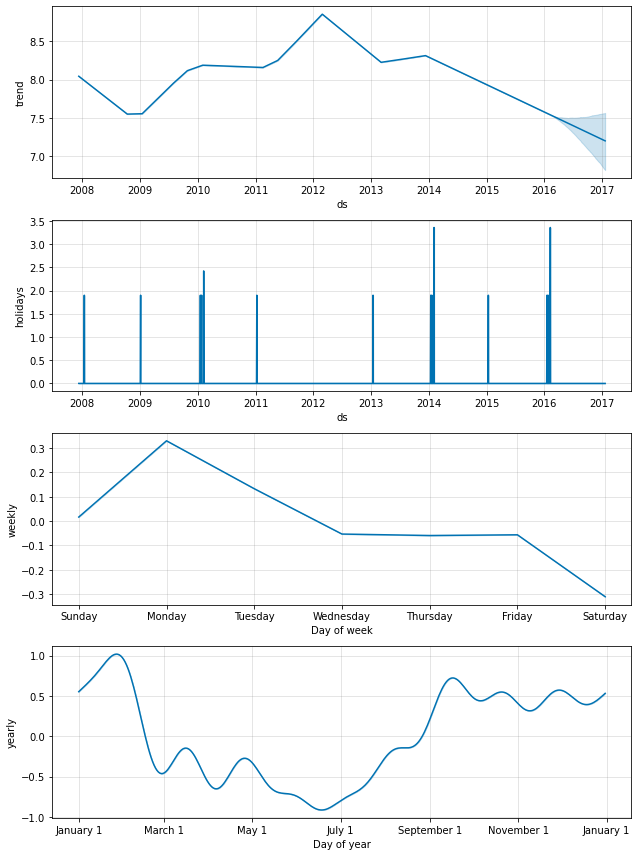
可以使用 plot_forecast_component 函数(从 Python 中的 prophet.plot 导入)绘制单个节假日,例如 plot_forecast_component(m, forecast, 'superbowl') 来绘制超级碗节假日成分。
内置国家节假日
您可以使用 add_country_holidays 方法(Python)或函数(R)来使用内置的特定国家/地区的节假日集合。 指定国家/地区的名称,然后除了通过上述 holidays 参数指定的任何节假日之外,还将包括该国家/地区的主要节假日。
1
2
3
4
# R
m <- prophet(holidays = holidays)
m <- add_country_holidays(m, country_name = 'US')
m <- fit.prophet(m, df)
1
2
3
4
# Python
m = Prophet(holidays=holidays)
m.add_country_holidays(country_name='US')
m.fit(df)
您可以通过查看模型的 train_holiday_names (Python) 或 train.holiday.names (R) 属性来查看包含哪些节假日。
1
2
# R
m$train.holiday.names
1
2
3
4
5
6
7
8
 [1] "playoff"                     "superbowl"
 [3] "New Year's Day"              "Martin Luther King Jr. Day"
 [5] "Washington's Birthday"       "Memorial Day"
 [7] "Independence Day"            "Labor Day"
 [9] "Columbus Day"                "Veterans Day"
[11] "Veterans Day (Observed)"     "Thanksgiving"
[13] "Christmas Day"               "Independence Day (Observed)"
[15] "Christmas Day (Observed)"    "New Year's Day (Observed)"
1
2
# Python
m.train_holiday_names
1
2
3
4
5
6
7
8
9
10
11
12
13
14
15
16
17
0                         playoff
1                       superbowl
2                  New Year's Day
3      Martin Luther King Jr. Day
4           Washington's Birthday
5                    Memorial Day
6                Independence Day
7                       Labor Day
8                    Columbus Day
9                    Veterans Day
10                   Thanksgiving
11                  Christmas Day
12       Christmas Day (Observed)
13        Veterans Day (Observed)
14    Independence Day (Observed)
15      New Year's Day (Observed)
dtype: object
每个国家/地区的节假日由 Python 中的 holidays 包提供。 可用国家/地区的列表以及要使用的国家/地区名称可在其页面上找到:https://github.com/vacanza/python-holidays/。
在 Python 中,大多数节假日都是确定性计算的,因此可用于任何日期范围;如果日期超出该国家/地区支持的范围,将发出警告。 在 R 中,计算了 1995 年至 2044 年的节假日日期,并作为 data-raw/generated_holidays.csv 存储在该包中。 如果需要更宽的日期范围,可以使用此脚本将该文件替换为不同的日期范围:https://github.com/facebook/prophet/blob/main/python/scripts/generate_holidays_file.py。
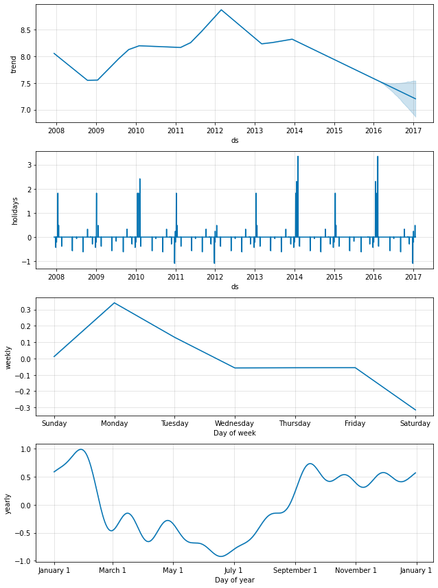
如上所述,国家/地区级别的节假日将显示在成分图中。
1
2
3
# R
forecast <- predict(m, future)
prophet_plot_components(m, forecast)
1
2
3
# Python
forecast = m.predict(future)
fig = m.plot_components(forecast)
细分区域的节假日 (Python)
我们可以使用实用函数 make_holidays_df 轻松创建自定义节假日 DataFrames,例如,使用来自 holidays 包的数据用于某些州。 这可以直接传递给 Prophet() 构造函数。
1
2
3
4
5
6
7
# Python
from prophet.make_holidays import make_holidays_df

nsw_holidays = make_holidays_df(
    year_list=[2019 + i for i in range(10)], country='AU', province='NSW'
)
nsw_holidays.head(n=10)
| ds | holiday | |
|---|---|---|
| 0 | 2019-01-26 | Australia Day |
| 1 | 2019-01-28 | Australia Day (Observed) |
| 2 | 2019-04-25 | Anzac Day |
| 3 | 2019-12-25 | Christmas Day |
| 4 | 2019-12-26 | Boxing Day |
| 5 | 2019-04-20 | Easter Saturday |
| 6 | 2019-04-21 | Easter Sunday |
| 7 | 2019-10-07 | Labour Day |
| 8 | 2019-06-10 | Queen's Birthday |
| 9 | 2019-08-05 | Bank Holiday |
1
2
3
4
# Python
from prophet import Prophet

m_nsw = Prophet(holidays=nsw_holidays)
季节性的傅里叶阶数
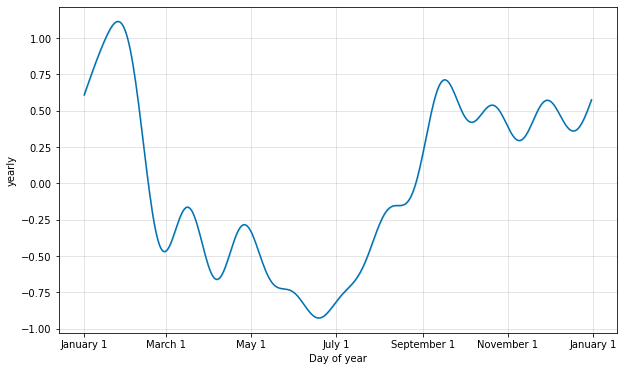
季节性是使用部分傅里叶和估计的。 有关完整详细信息,请参见论文,并参见维基百科上的这张图,以说明部分傅里叶和如何逼近任意周期信号。 部分和中的项数(阶数)是一个参数,用于确定季节性可以变化的速度。 为了说明这一点,请考虑来自 快速入门的 Peyton Manning 数据。 年度季节性的默认傅里叶阶数为 10,产生如下拟合。
1
2
3
# R
m <- prophet(df)
prophet:::plot_yearly(m)
1
2
3
4
# Python
from prophet.plot import plot_yearly
m = Prophet().fit(df)
a = plot_yearly(m)
默认值通常是合适的,但是当季节性需要拟合更高频率的变化时,可以增加这些值,并且通常不太平滑。 在实例化模型时,可以为每个内置的季节性指定傅里叶阶数,在这里将其增加到 20。
1
2
3
# R
m <- prophet(df, yearly.seasonality = 20)
prophet:::plot_yearly(m)
1
2
3
4
# Python
from prophet.plot import plot_yearly
m = Prophet(yearly_seasonality=20).fit(df)
a = plot_yearly(m)
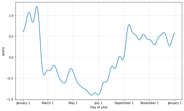
增加傅里叶项数允许季节性拟合更快变化的周期,但也可能导致过度拟合:N 个傅里叶项对应于用于建模周期的 2N 个变量。
指定自定义季节性
如果时间序列超过两个周期,Prophet 默认会拟合每周和每年的季节性。 它还将为亚每日时间序列拟合每日季节性。 您可以使用 add_seasonality 方法(Python)或函数(R)添加其他季节性(每月、每季度、每小时)。
此函数的输入是名称、季节性的周期(以天为单位)和季节性的傅里叶阶数。 作为参考,默认情况下,Prophet 对每周季节性使用 3 的傅里叶阶数,对年度季节性使用 10 的傅里叶阶数。 add_seasonality 的一个可选输入是该季节性成分的先验尺度 - 这将在下面讨论。
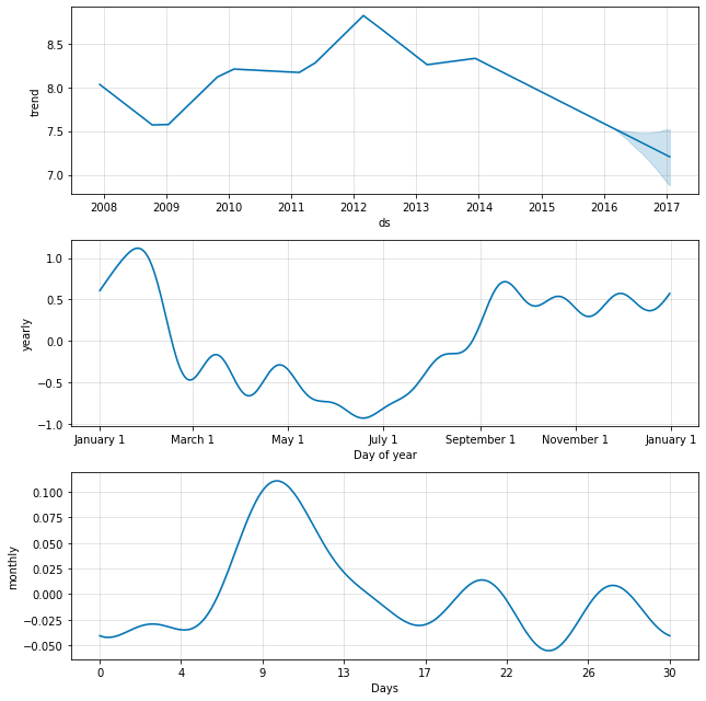
例如,在这里,我们拟合了来自 快速入门的 Peyton Manning 数据,但用每月季节性代替了每周季节性。 然后,每月季节性将出现在成分图中。
1
2
3
4
5
6
# R
m <- prophet(weekly.seasonality=FALSE)
m <- add_seasonality(m, name='monthly', period=30.5, fourier.order=5)
m <- fit.prophet(m, df)
forecast <- predict(m, future)
prophet_plot_components(m, forecast)
1
2
3
4
5
# Python
m = Prophet(weekly_seasonality=False)
m.add_seasonality(name='monthly', period=30.5, fourier_order=5)
forecast = m.fit(df).predict(future)
fig = m.plot_components(forecast)
取决于其他因素的季节性
在某些情况下,季节性可能取决于其他因素,例如夏季的每周季节性模式与一年中其他时间的每周季节性模式不同,或者周末的每日季节性模式与工作日的每日季节性模式不同。 这些类型的季节性可以使用条件季节性进行建模。
考虑来自 快速入门的 Peyton Manning 示例。 默认的每周季节性假设每周季节性的模式在全年都是相同的,但是我们希望每周季节性的模式在赛季(每个星期天都有比赛时)和休赛期是不同的。 我们可以使用条件季节性来构建单独的赛季和休赛期每周季节性。
首先,我们向数据框添加一个布尔列,指示每个日期是否在赛季或休赛期。
1
2
3
4
5
6
7
8
# R
is_nfl_season <- function(ds) {
  dates <- as.Date(ds)
  month <- as.numeric(format(dates, '%m'))
  return(month > 8 | month < 2)
}
df$on_season <- is_nfl_season(df$ds)
df$off_season <- !is_nfl_season(df$ds)
1
2
3
4
5
6
7
# Python
def is_nfl_season(ds):
    date = pd.to_datetime(ds)
    return (date.month > 8 or date.month < 2)

df['on_season'] = df['ds'].apply(is_nfl_season)
df['off_season'] = ~df['ds'].apply(is_nfl_season)
然后,我们禁用内置的每周季节性,并用两个每周季节性代替它,这两个每周季节性将这些列指定为条件。 这意味着季节性将仅应用于 condition_name 列为 True 的日期。 我们还必须将该列添加到我们要进行预测的 future 数据框中。
1
2
3
4
5
6
7
8
9
10
# R
m <- prophet(weekly.seasonality=FALSE)
m <- add_seasonality(m, name='weekly_on_season', period=7, fourier.order=3, condition.name='on_season')
m <- add_seasonality(m, name='weekly_off_season', period=7, fourier.order=3, condition.name='off_season')
m <- fit.prophet(m, df)

future$on_season <- is_nfl_season(future$ds)
future$off_season <- !is_nfl_season(future$ds)
forecast <- predict(m, future)
prophet_plot_components(m, forecast)
1
2
3
4
5
6
7
8
9
# Python
m = Prophet(weekly_seasonality=False)
m.add_seasonality(name='weekly_on_season', period=7, fourier_order=3, condition_name='on_season')
m.add_seasonality(name='weekly_off_season', period=7, fourier_order=3, condition_name='off_season')

future['on_season'] = future['ds'].apply(is_nfl_season)
future['off_season'] = ~future['ds'].apply(is_nfl_season)
forecast = m.fit(df).predict(future)
fig = m.plot_components(forecast)
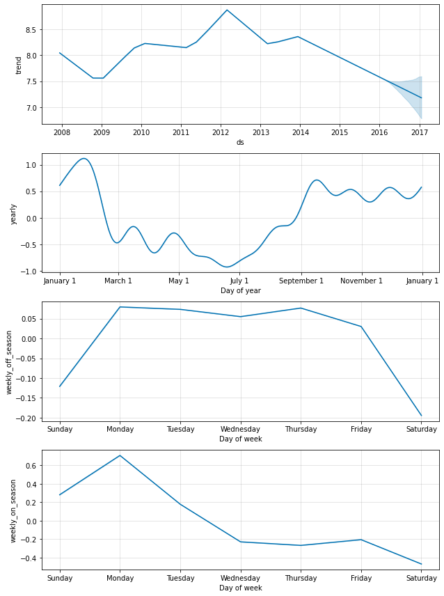
现在,两种季节性都显示在上面的成分图中。 我们可以看到,在赛季期间,每个星期天都有比赛,星期天和星期一都会大幅增加,而在休赛期则完全没有。
节假日和季节性的先验尺度
如果您发现节假日过度拟合,则可以使用参数 holidays_prior_scale 调整其先验尺度以使其平滑。 默认情况下,此参数为 10,提供的正则化很少。 减少此参数会抑制节假日效应。
1
2
3
4
5
6
7
# R
m <- prophet(df, holidays = holidays, holidays.prior.scale = 0.05)
forecast <- predict(m, future)
forecast %>%
  select(ds, playoff, superbowl) %>%
  filter(abs(playoff + superbowl) > 0) %>%
  tail(10)
1
2
3
4
5
# Python
m = Prophet(holidays=holidays, holidays_prior_scale=0.05).fit(df)
forecast = m.predict(future)
forecast[(forecast['playoff'] + forecast['superbowl']).abs() > 0][
    ['ds', 'playoff', 'superbowl']][-10:]
| ds | playoff | superbowl | |
|---|---|---|---|
| 2190 | 2014-02-02 | 1.206086 | 0.964914 |
| 2191 | 2014-02-03 | 1.852077 | 0.992634 |
| 2532 | 2015-01-11 | 1.206086 | 0.000000 |
| 2533 | 2015-01-12 | 1.852077 | 0.000000 |
| 2901 | 2016-01-17 | 1.206086 | 0.000000 |
| 2902 | 2016-01-18 | 1.852077 | 0.000000 |
| 2908 | 2016-01-24 | 1.206086 | 0.000000 |
| 2909 | 2016-01-25 | 1.852077 | 0.000000 |
| 2922 | 2016-02-07 | 1.206086 | 0.964914 |
| 2923 | 2016-02-08 | 1.852077 | 0.992634 |
与之前相比,节假日效应的幅度已减小,尤其是对于观测值最少的超级碗。 还有一个参数 seasonality_prior_scale,它类似地调整季节性模型拟合数据的程度。
可以通过在节假日数据框中包含列 prior_scale 来为单个节假日分别设置先验尺度。 可以将单个季节性的先验尺度作为参数传递给 add_seasonality。 例如,可以使用以下命令设置仅每周季节性的先验尺度
1
2
3
4
# R
m <- prophet()
m <- add_seasonality(
  m, name='weekly', period=7, fourier.order=3, prior.scale=0.1)
1
2
3
4
# Python
m = Prophet()
m.add_seasonality(
    name='weekly', period=7, fourier_order=3, prior_scale=0.1)
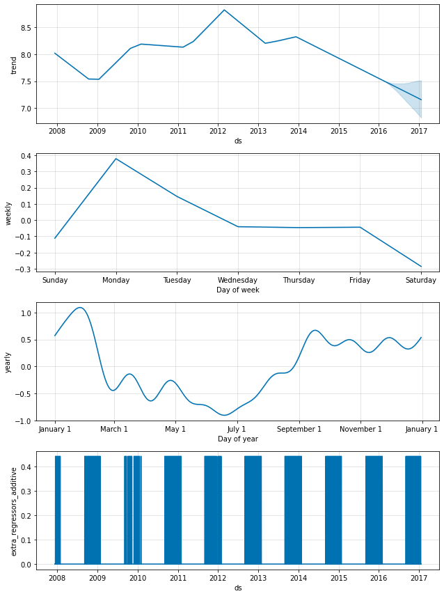
附加回归变量
可以使用 add_regressor 方法或函数将其他回归变量添加到模型的线性部分。 回归变量值的列需要存在于拟合和预测数据框中。 例如,我们可以添加 NFL 赛季期间星期天的其他影响。 在成分图中,此影响将显示在“extra_regressors”图中。
1
2
3
4
5
6
7
8
9
10
11
12
13
14
15
16
# R
nfl_sunday <- function(ds) {
  dates <- as.Date(ds)
  month <- as.numeric(format(dates, '%m'))
  as.numeric((weekdays(dates) == "Sunday") & (month > 8 | month < 2))
}
df$nfl_sunday <- nfl_sunday(df$ds)

m <- prophet()
m <- add_regressor(m, 'nfl_sunday')
m <- fit.prophet(m, df)

future$nfl_sunday <- nfl_sunday(future$ds)

forecast <- predict(m, future)
prophet_plot_components(m, forecast)
1
2
3
4
5
6
7
8
9
10
11
12
13
14
15
16
17
# Python
def nfl_sunday(ds):
    date = pd.to_datetime(ds)
    if date.weekday() == 6 and (date.month > 8 or date.month < 2):
        return 1
    else:
        return 0
df['nfl_sunday'] = df['ds'].apply(nfl_sunday)

m = Prophet()
m.add_regressor('nfl_sunday')
m.fit(df)

future['nfl_sunday'] = future['ds'].apply(nfl_sunday)

forecast = m.predict(future)
fig = m.plot_components(forecast)
也可以使用上述“节假日”界面来处理 NFL 星期天,方法是创建过去和将来的 NFL 星期天列表。 add_regressor 函数为定义额外的线性回归变量提供了一个更通用的界面,尤其是不要求回归变量是二元指标。 另一个时间序列可以用作回归变量,尽管必须知道其未来值。
此笔记本显示了使用天气因素作为自行车使用量预测中的额外回归变量的示例,并提供了一个很好的说明,说明了如何将其他时间序列包括为额外回归变量。
add_regressor 函数具有用于指定先验尺度(默认使用节假日先验尺度)以及是否标准化回归变量的可选参数 - 请参见 Python 中的 help(Prophet.add_regressor) 和 R 中的 ?add_regressor 的 docstring。 请注意,必须在模型拟合之前添加回归变量。 如果回归变量在整个历史记录中都是常数,Prophet 也会引发错误,因为没有任何可以拟合的内容。
额外的回归变量必须在历史数据和未来日期中都已知。因此,它必须是具有已知未来值的变量(例如 nfl_sunday),或者是在其他地方单独预测过的变量。上面链接的笔记本中使用的天气回归变量就是一个很好的例子,它具有可以用于未来值的预测值。
您还可以将另一个时间序列用作回归变量,该时间序列已使用时间序列模型(例如 Prophet)进行预测。例如,如果 r(t) 作为 y(t) 的回归变量,则可以使用 Prophet 预测 r(t),然后在预测 y(t) 时,将该预测值作为未来值插入。请注意,除非 r(t) 比 y(t) 更容易预测,否则此方法可能不会有用。这是因为对 r(t) 的预测误差会导致对 y(t) 的预测误差。这种方法可能有用的一种情况是在分层时间序列中,顶层预测具有更高的信噪比,因此更容易预测。它的预测可以包含在每个较低层级序列的预测中。
额外的回归变量被放置在模型的线性分量中,因此底层模型是时间序列以加性或乘性因子依赖于额外的回归变量(有关乘性的更多信息,请参见下一节)。
附加回归变量的系数
要提取额外的回归变量的 beta 系数,请使用实用程序函数 regressor_coefficients(在 Python 中为 from prophet.utilities import regressor_coefficients,在 R 中为 prophet::regressor_coefficients)对拟合模型进行操作。每个回归变量的估计 beta 系数大致表示回归变量值每增加一个单位,预测值增加的量(请注意,返回的系数始终是原始数据的规模)。如果指定了 mcmc_samples,还会返回每个系数的可信区间,这有助于识别回归变量对模型是否有意义(包含 0 值的可信区间表明回归变量没有意义)。