
非日度数据
亚日数据
Prophet 可以通过传入一个包含时间戳的 ds 列的数据框来为具有亚日观测值的时间序列进行预测。时间戳的格式应该是 YYYY-MM-DD HH:MM:SS - 请参阅此处的示例 csv here。当使用亚日数据时,将自动拟合每日季节性。这里我们将 Prophet 拟合到具有 5 分钟分辨率的数据(Yosemite 的每日温度)
1
2
3
4
5
6
# R
df <- read.csv('https://raw.githubusercontent.com/facebook/prophet/main/examples/example_yosemite_temps.csv')
m <- prophet(df, changepoint.prior.scale=0.01)
future <- make_future_dataframe(m, periods = 300, freq = 60 * 60)
fcst <- predict(m, future)
plot(m, fcst)
1
2
3
4
5
6
# Python
df = pd.read_csv('https://raw.githubusercontent.com/facebook/prophet/main/examples/example_yosemite_temps.csv')
m = Prophet(changepoint_prior_scale=0.01).fit(df)
future = m.make_future_dataframe(periods=300, freq='H')
fcst = m.predict(future)
fig = m.plot(fcst)
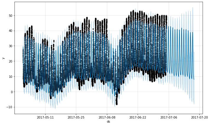
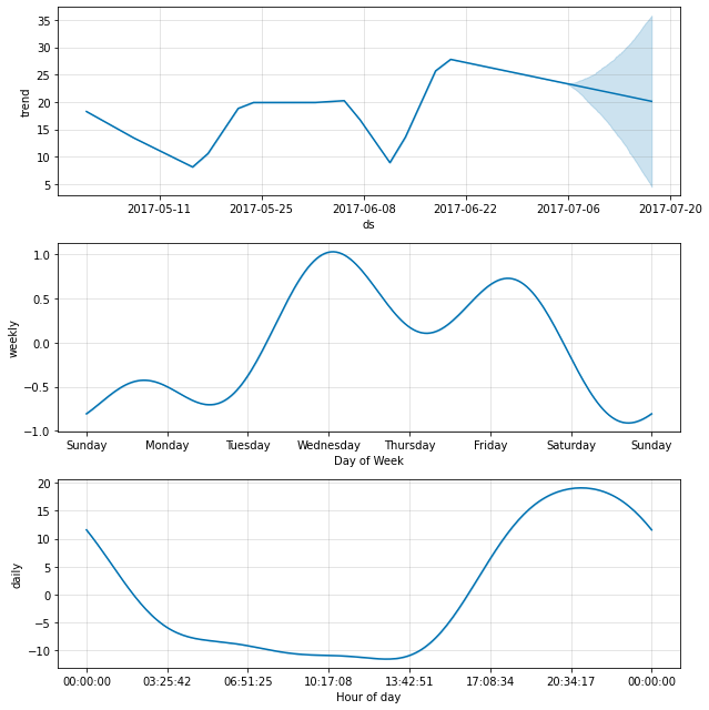
每日季节性将显示在分量图中
1
2
# R
prophet_plot_components(m, fcst)
1
2
# Python
fig = m.plot_components(fcst)
具有规律间隔的数据
假设上面的数据集只有从凌晨 12 点到早上 6 点的观测值
1
2
3
4
5
6
7
8
# R
df2 <- df %>%
  mutate(ds = as.POSIXct(ds, tz="GMT")) %>%
  filter(as.numeric(format(ds, "%H")) < 6)
m <- prophet(df2)
future <- make_future_dataframe(m, periods = 300, freq = 60 * 60)
fcst <- predict(m, future)
plot(m, fcst)
1
2
3
4
5
6
7
8
# Python
df2 = df.copy()
df2['ds'] = pd.to_datetime(df2['ds'])
df2 = df2[df2['ds'].dt.hour < 6]
m = Prophet().fit(df2)
future = m.make_future_dataframe(periods=300, freq='H')
fcst = m.predict(future)
fig = m.plot(fcst)
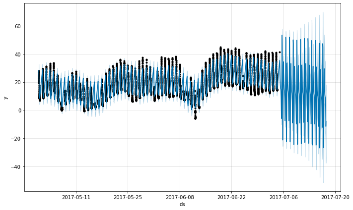
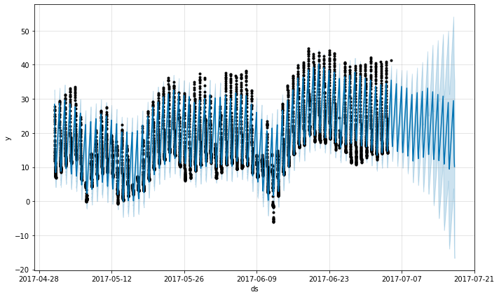
预测看起来非常糟糕,未来的波动比历史上看到的要大得多。这里的问题是我们已经将每日周期拟合到仅包含一天中一部分数据(凌晨 12 点到早上 6 点)的时间序列。因此,对于一天中的剩余时间,每日季节性不受约束,并且估计不佳。解决方案是仅对存在历史数据的时间窗口进行预测。在这里,这意味着限制 future 数据框,使其具有凌晨 12 点到早上 6 点的时间
1
2
3
4
5
# R
future2 <- future %>%
  filter(as.numeric(format(ds, "%H")) < 6)
fcst <- predict(m, future2)
plot(m, fcst)
1
2
3
4
5
# Python
future2 = future.copy()
future2 = future2[future2['ds'].dt.hour < 6]
fcst = m.predict(future2)
fig = m.plot(fcst)
同样的原则适用于数据中存在规律间隔的其他数据集。例如,如果历史记录仅包含工作日,那么应该仅对工作日进行预测,因为周末的每周季节性将无法得到很好的估计。
月度数据
您可以使用 Prophet 来拟合月度数据。但是,底层模型是连续时间的,这意味着如果您将模型拟合到月度数据,然后要求进行每日预测,您可能会得到奇怪的结果。在这里,我们预测未来 10 年的美国零售额
1
2
3
4
5
6
# R
df <- read.csv('https://raw.githubusercontent.com/facebook/prophet/main/examples/example_retail_sales.csv')
m <- prophet(df, seasonality.mode = 'multiplicative')
future <- make_future_dataframe(m, periods = 3652)
fcst <- predict(m, future)
plot(m, fcst)
1
2
3
4
5
6
# Python
df = pd.read_csv('https://raw.githubusercontent.com/facebook/prophet/main/examples/example_retail_sales.csv')
m = Prophet(seasonality_mode='multiplicative').fit(df)
future = m.make_future_dataframe(periods=3652)
fcst = m.predict(future)
fig = m.plot(fcst)
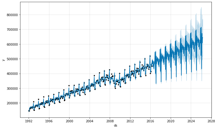
这与上面数据集具有规律间隔的问题相同。当我们拟合年度季节性时,它只有每个月第一天的数据,剩余日子的季节性分量是无法识别和过度拟合的。通过进行 MCMC 以查看季节性的不确定性,可以清楚地看到这一点
1
2
3
4
# R
m <- prophet(df, seasonality.mode = 'multiplicative', mcmc.samples = 300)
fcst <- predict(m, future)
prophet_plot_components(m, fcst)
1
2
3
4
# Python
m = Prophet(seasonality_mode='multiplicative', mcmc_samples=300).fit(df, show_progress=False)
fcst = m.predict(future)
fig = m.plot_components(fcst)
1
2
WARNING:pystan:481 of 600 iterations saturated the maximum tree depth of 10 (80.2 %)
WARNING:pystan:Run again with max_treedepth larger than 10 to avoid saturation
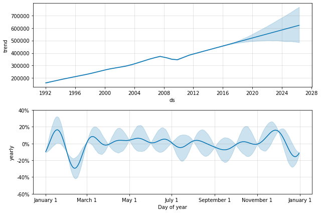
季节性在每个月开始时数据点所在的位置的不确定性较低,但在两者之间的后验方差非常高。将 Prophet 拟合到月度数据时,仅进行月度预测,这可以通过将频率传递到 make_future_dataframe 中来完成
1
2
3
4
# R
future <- make_future_dataframe(m, periods = 120, freq = 'month')
fcst <- predict(m, future)
plot(m, fcst)
1
2
3
4
# Python
future = m.make_future_dataframe(periods=120, freq='MS')
fcst = m.predict(future)
fig = m.plot(fcst)
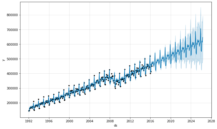
在 Python 中,频率可以是 pandas 频率字符串列表中的任何值,请参见:https://pandas.ac.cn/pandas-docs/stable/user_guide/timeseries.html#timeseries-offset-aliases 。请注意,此处使用的 MS 是 month-start,表示数据点放置在每个月的开始。
在月度数据中,也可以使用二元附加回归变量对年度季节性进行建模。特别是,该模型可以使用 12 个额外的回归变量,例如 is_jan、is_feb 等,其中如果日期在 1 月,则 is_jan 为 1,否则为 0。这种方法可以避免上面看到的月份内的不可识别性。如果添加了月度附加回归变量,请务必使用 yearly_seasonality=False。
具有聚合数据的假日
假日效应应用于指定假日的特定日期。对于已聚合到每周或每月频率的数据,如果假日没有落在数据中使用的特定日期,则将忽略这些假日:例如,每周时间序列中的星期一假日,其中每个数据点都在星期日。要在模型中包含假日效应,需要将假日移动到历史数据框中想要效应的日期。请注意,对于每周或每月聚合的数据,许多假日效应将被年度季节性很好地捕获,因此只有在整个时间序列中发生在不同周的假日才需要添加假日。