
其他主题
保存模型
可以保存拟合的 Prophet 模型,以便稍后加载和使用。
在 R 中,这是通过 saveRDS 和 readRDS 完成的
1
2
3
# R
saveRDS(m, file="model.RDS")  # Save model
m <- readRDS(file="model.RDS")  # Load model
在 Python 中,不应使用 pickle 保存模型;附加到模型对象的 Stan 后端无法很好地进行 pickle,并且会在某些 Python 版本下产生问题。 相反,您应该使用内置的序列化函数将模型序列化为 json
1
2
3
4
5
6
7
8
# Python
from prophet.serialize import model_to_json, model_from_json

with open('serialized_model.json', 'w') as fout:
    fout.write(model_to_json(m))  # Save model

with open('serialized_model.json', 'r') as fin:
    m = model_from_json(fin.read())  # Load model
json 文件将在系统之间可移植,并且反序列化与旧版本的 prophet 向后兼容。
平坦趋势
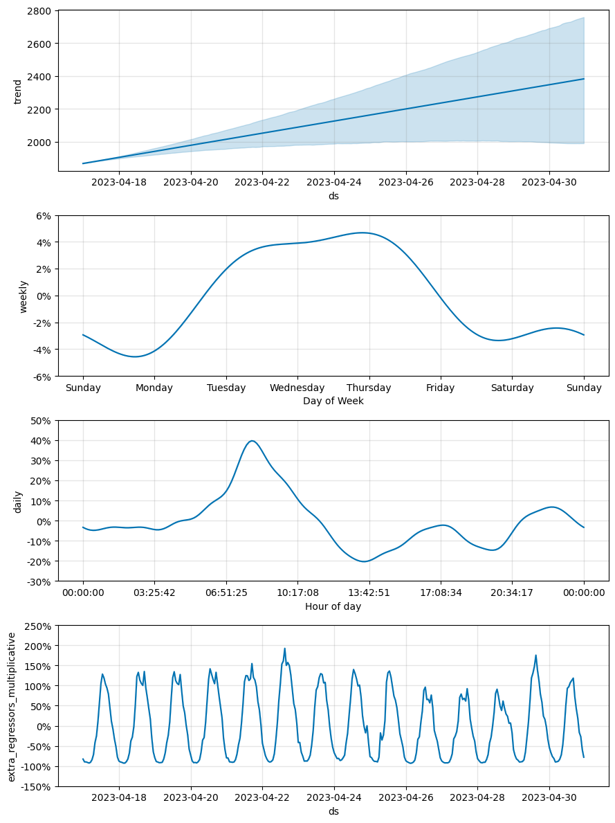
对于表现出强季节性模式而不是趋势变化的时间序列,或者当我们想要依赖外生回归量的模式时(例如,用于时间序列的因果推理),强制趋势增长率为平坦可能很有用。 这可以通过在创建模型时简单地传递 growth='flat' 来实现
1
2
# R
m <- prophet(df, growth='flat')
1
2
# Python
m = Prophet(growth='flat')
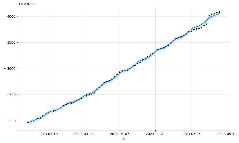
下面是使用线性增长与平坦增长使用外生回归量进行反事实预测的比较。
1
2
3
4
5
6
7
8
9
10
11
12
13
14
15
16
17
18
19
20
21
# Python
import pandas as pd
from prophet import Prophet
import matplotlib.pyplot as plt

import warnings
warnings.simplefilter(action='ignore', category=FutureWarning)

regressor = "location_4"
target = "location_41"
cutoff = pd.to_datetime("2023-04-17 00:00:00")

df = (
    pd.read_csv(
        "https://raw.githubusercontent.com/facebook/prophet/main/examples/example_pedestrians_multivariate.csv",
        parse_dates=["ds"]
    )
    .rename(columns={target: "y"})
)
train = df.loc[df["ds"] < cutoff]
test = df.loc[df["ds"] >= cutoff]
1
2
3
4
5
6
7
8
9
10
11
12
13
# Python
def fit_model(growth):
    m = Prophet(growth=growth, seasonality_mode="multiplicative", daily_seasonality=15)
    m.add_regressor("location_4", mode="multiplicative")
    m.fit(train)
    preds = pd.merge(
        test,
        m.predict(test),
        on="ds",
        how="inner"
    )
    mape = ((preds["yhat"] - preds["y"]).abs() / preds_linear["y"]).mean()
    return m, preds, mape
1
2
# Python
m_linear, preds_linear, mape_linear = fit_model("linear")
1
2
01:19:58 - cmdstanpy - INFO - Chain [1] start processing
01:19:58 - cmdstanpy - INFO - Chain [1] done processing
1
2
# Python
m_flat, preds_flat, mape_flat = fit_model("flat")
1
2
01:19:58 - cmdstanpy - INFO - Chain [1] start processing
01:19:58 - cmdstanpy - INFO - Chain [1] done processing
1
2
# Python
m_linear.plot_components(preds_linear);
1
2
# Python
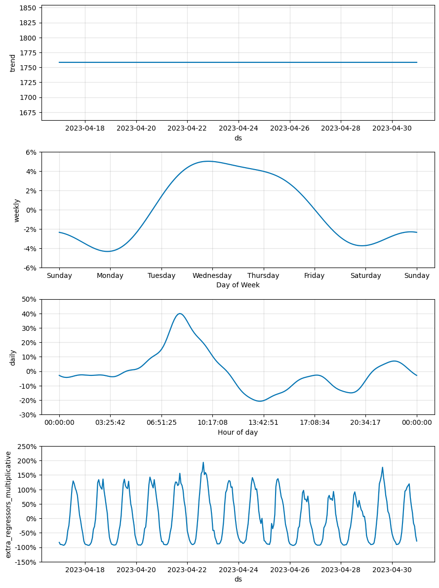
m_flat.plot_components(preds_flat);
1
2
3
4
5
6
7
# Python
fig, ax = plt.subplots(figsize=(11, 5))
ax.scatter(preds_linear["ds"], preds_linear["y"], color="black", marker=".")
ax.plot(preds_linear["ds"], preds_linear["yhat"], label=f"linear, mape={mape_linear:.1%}")
ax.plot(preds_flat["ds"], preds_flat["yhat"], label=f"flat, mape={mape_flat:.1%}")
plt.xticks(rotation=60)
ax.legend();
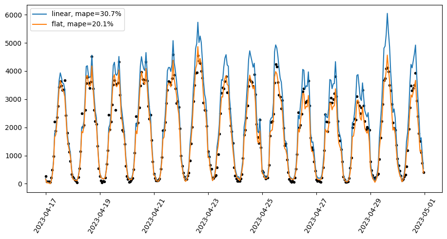
在此示例中,目标传感器值可以通过外生回归量(附近的传感器)来解释。 具有线性增长的模型假设趋势增加,这导致测试期间越来越大的过度预测,而平坦增长模型主要遵循外生回归量的移动,这导致了显着的 MAPE 改进。
请注意,仅当我们对外生回归量的未来值有信心时,使用外生回归量进行预测才有效。 上面的示例与使用时间序列进行因果推理相关,我们想了解过去一段时间内的 y 是什么样子的,因此外生回归量值是已知的。
在其他情况下——当我们没有外生回归量或必须预测它们的未来值时——如果在没有恒定趋势的时间序列上使用平坦增长,任何趋势都将与噪声项拟合,因此预测中的预测不确定性会很高。
自定义趋势
要使用这三种内置趋势函数(分段线性、分段逻辑增长和平面)之外的趋势,您可以从 github 下载源代码,在本地分支中根据需要修改趋势函数,然后安装该本地版本。 此 PR 很好地说明了实现自定义趋势必须要做什么,这一个实现了阶跃函数趋势,这一个实现了 R 中的新趋势。
更新拟合模型
预测的一个常见设置是拟合需要随着额外数据的进入而更新的模型。 Prophet 模型只能拟合一次,并且当有新数据可用时,必须重新拟合新模型。 在大多数情况下,模型拟合速度足够快,重新从头开始拟合没有任何问题。 但是,可以通过从早期模型的模型参数中预热启动拟合来稍微加快速度。 此代码示例显示了如何在 Python 中执行此操作
1
2
3
4
5
6
7
8
9
10
11
12
13
14
15
16
17
18
19
20
21
22
23
24
25
26
27
28
29
30
31
32
33
34
35
36
# Python
def warm_start_params(m):
    """
    Retrieve parameters from a trained model in the format used to initialize a new Stan model.
    Note that the new Stan model must have these same settings:
        n_changepoints, seasonality features, mcmc sampling
    for the retrieved parameters to be valid for the new model.

    Parameters
    ----------
    m: A trained model of the Prophet class.

    Returns
    -------
    A Dictionary containing retrieved parameters of m.
    """
    res = {}
    for pname in ['k', 'm', 'sigma_obs']:
        if m.mcmc_samples == 0:
            res[pname] = m.params[pname][0][0]
        else:
            res[pname] = np.mean(m.params[pname])
    for pname in ['delta', 'beta']:
        if m.mcmc_samples == 0:
            res[pname] = m.params[pname][0]
        else:
            res[pname] = np.mean(m.params[pname], axis=0)
    return res

df = pd.read_csv('https://raw.githubusercontent.com/facebook/prophet/main/examples/example_wp_log_peyton_manning.csv')
df1 = df.loc[df['ds'] < '2016-01-19', :]  # All data except the last day
m1 = Prophet().fit(df1) # A model fit to all data except the last day


%timeit m2 = Prophet().fit(df)  # Adding the last day, fitting from scratch
%timeit m2 = Prophet().fit(df, init=warm_start_params(m1))  # Adding the last day, warm-starting from m1
1
2
1.33 s ± 55.9 ms per loop (mean ± std. dev. of 7 runs, 1 loop each)
185 ms ± 4.46 ms per loop (mean ± std. dev. of 7 runs, 10 loops each)
可以看出,先前模型中的参数与 kwarg init 一起传递到下一个模型的拟合中。 在这种情况下,使用热启动时,模型拟合速度快了约 5 倍。 加速通常取决于最佳模型参数随新数据的添加而变化多少。
在考虑热启动时,应记住一些注意事项。 首先,热启动对于数据的少量更新(如上面示例中添加的一天)可能效果很好,但如果数据发生重大变化(即,添加了大量天数),则可能比从头开始拟合更糟。 这是因为当添加大量历史记录时,两个模型之间变化点的位置将非常不同,因此先前模型中的参数实际上可能会产生错误的趋势初始化。 其次,作为一个细节,变化点的数量需要从一个模型到下一个模型保持一致,否则会引发错误,因为变化点先验参数 delta 的大小将不正确。
minmax 缩放 (1.1.5 中的新功能)
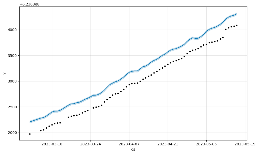
在模型拟合之前,Prophet 通过将 y 除以历史记录中的最大值来缩放 y。 对于具有非常大的 y 值的数据集,缩放后的 y 值可能会被压缩到非常小的范围内(即 [0.99999... - 1.0]),这会导致拟合不良。 可以通过在 Prophet 构造函数中设置 scaling='minmax' 来解决此问题。
1
2
3
4
5
# Python
large_y = pd.read_csv(
    "https://raw.githubusercontent.com/facebook/prophet/main/python/prophet/tests/data3.csv",
    parse_dates=["ds"]
)
1
2
3
# Python
m1 = Prophet(scaling="absmax")
m1 = m1.fit(large_y)
1
2
08:11:23 - cmdstanpy - INFO - Chain [1] start processing
08:11:23 - cmdstanpy - INFO - Chain [1] done processing
1
2
3
# Python
m2 = Prophet(scaling="minmax")
m2 = m2.fit(large_y)
1
2
08:11:29 - cmdstanpy - INFO - Chain [1] start processing
08:11:29 - cmdstanpy - INFO - Chain [1] done processing
1
2
# Python
m1.plot(m1.predict(large_y));
1
2
# Python
m2.plot(m2.predict(large_y));
检查转换后的数据 (1.1.5 中的新功能)
对于调试,了解原始数据在传递给 stan 拟合例程之前是如何转换的很有用。 我们可以调用 .preprocess() 方法来查看 stan 的所有输入,并调用 .calculate_init_params() 来查看模型参数将如何初始化。
1
2
3
4
# Python
df = pd.read_csv('https://raw.githubusercontent.com/facebook/prophet/main/examples/example_wp_log_peyton_manning.csv')
m = Prophet()
transformed = m.preprocess(df)
1
2
# Python
transformed.y.head(n=10)
1
2
3
4
5
6
7
8
9
10
11
0    0.746552
1    0.663171
2    0.637023
3    0.628367
4    0.614441
5    0.605884
6    0.654956
7    0.687273
8    0.652501
9    0.628148
Name: y_scaled, dtype: float64
1
2
# Python
transformed.X.head(n=10)
| yearly_delim_1 | yearly_delim_2 | yearly_delim_3 | yearly_delim_4 | yearly_delim_5 | yearly_delim_6 | yearly_delim_7 | yearly_delim_8 | yearly_delim_9 | yearly_delim_10 | ... | yearly_delim_17 | yearly_delim_18 | yearly_delim_19 | yearly_delim_20 | weekly_delim_1 | weekly_delim_2 | weekly_delim_3 | weekly_delim_4 | weekly_delim_5 | weekly_delim_6 | |
|---|---|---|---|---|---|---|---|---|---|---|---|---|---|---|---|---|---|---|---|---|---|
| 0 | -0.377462 | 0.926025 | -0.699079 | 0.715044 | -0.917267 | 0.398272 | -0.999745 | 0.022576 | -0.934311 | -0.356460 | ... | 0.335276 | -0.942120 | 0.666089 | -0.745872 | -4.338837e-01 | -0.900969 | 7.818315e-01 | 0.623490 | -9.749279e-01 | -0.222521 |
| 1 | -0.361478 | 0.932381 | -0.674069 | 0.738668 | -0.895501 | 0.445059 | -0.995827 | 0.091261 | -0.961479 | -0.274879 | ... | 0.185987 | -0.982552 | 0.528581 | -0.848883 | -9.749279e-01 | -0.222521 | 4.338837e-01 | -0.900969 | 7.818315e-01 | 0.623490 |
| 2 | -0.345386 | 0.938461 | -0.648262 | 0.761418 | -0.871351 | 0.490660 | -0.987196 | 0.159513 | -0.981538 | -0.191266 | ... | 0.032249 | -0.999480 | 0.375470 | -0.926834 | -7.818315e-01 | 0.623490 | -9.749279e-01 | -0.222521 | -4.338837e-01 | -0.900969 |
| 3 | -0.329192 | 0.944263 | -0.621687 | 0.783266 | -0.844881 | 0.534955 | -0.973892 | 0.227011 | -0.994341 | -0.106239 | ... | -0.122261 | -0.992498 | 0.211276 | -0.977426 | 5.505235e-14 | 1.000000 | 1.101047e-13 | 1.000000 | 1.984146e-12 | 1.000000 |
| 4 | -0.312900 | 0.949786 | -0.594376 | 0.804187 | -0.816160 | 0.577825 | -0.955979 | 0.293434 | -0.999791 | -0.020426 | ... | -0.273845 | -0.961774 | 0.040844 | -0.999166 | 7.818315e-01 | 0.623490 | 9.749279e-01 | -0.222521 | 4.338837e-01 | -0.900969 |
| 5 | -0.296516 | 0.955028 | -0.566362 | 0.824157 | -0.785267 | 0.619157 | -0.933542 | 0.358468 | -0.997850 | 0.065537 | ... | -0.418879 | -0.908042 | -0.130793 | -0.991410 | 9.749279e-01 | -0.222521 | -4.338837e-01 | -0.900969 | -7.818315e-01 | 0.623490 |
| 6 | -0.280044 | 0.959987 | -0.537677 | 0.843151 | -0.752283 | 0.658840 | -0.906686 | 0.421806 | -0.988531 | 0.151016 | ... | -0.553893 | -0.832588 | -0.298569 | -0.954388 | 4.338837e-01 | -0.900969 | -7.818315e-01 | 0.623490 | 9.749279e-01 | -0.222521 |
| 7 | -0.263489 | 0.964662 | -0.508356 | 0.861147 | -0.717295 | 0.696769 | -0.875539 | 0.483147 | -0.971904 | 0.235379 | ... | -0.675656 | -0.737217 | -0.457531 | -0.889193 | -4.338837e-01 | -0.900969 | 7.818315e-01 | 0.623490 | -9.749279e-01 | -0.222521 |
| 8 | -0.246857 | 0.969052 | -0.478434 | 0.878124 | -0.680398 | 0.732843 | -0.840248 | 0.542202 | -0.948090 | 0.318001 | ... | -0.781257 | -0.624210 | -0.602988 | -0.797750 | -9.749279e-01 | -0.222521 | 4.338837e-01 | -0.900969 | 7.818315e-01 | 0.623490 |
| 9 | -0.230151 | 0.973155 | -0.447945 | 0.894061 | -0.641689 | 0.766965 | -0.800980 | 0.598691 | -0.917267 | 0.398272 | ... | -0.868168 | -0.496271 | -0.730644 | -0.682758 | -7.818315e-01 | 0.623490 | -9.749279e-01 | -0.222521 | -4.338837e-01 | -0.900969 |
10 行 × 26 列
1
2
# Python
m.calculate_initial_params(num_total_regressors=transformed.K)
1
2
3
ModelParams(k=-0.05444079622224118, m=0.7465517318876905, delta=array([0., 0., 0., 0., 0., 0., 0., 0., 0., 0., 0., 0., 0., 0., 0., 0., 0.,
       0., 0., 0., 0., 0., 0., 0., 0.]), beta=array([0., 0., 0., 0., 0., 0., 0., 0., 0., 0., 0., 0., 0., 0., 0., 0., 0.,
       0., 0., 0., 0., 0., 0., 0., 0., 0.]), sigma_obs=1.0)
外部参考
正如我们在关于 Prophet 状态的 2023 年博客文章中讨论的那样,我们没有计划进一步开发底层的 Prophet 模型。 如果您正在寻找最先进的预测准确性,我们推荐以下库
-
statsforecast,以及来自 Nixtla 组的其他软件包,例如hierarchicalforecast和neuralforecast。 -
NeuralProphet,一种在 PyTorch 中实现的 Prophet 风格的模型,更具适应性和可扩展性。
这些 github 存储库提供了构建在 Prophet 之上的示例,这些示例可能具有广泛的兴趣
- forecastr:一个为 Prophet 提供 UI 的 Web 应用程序。